")
")


**By Isabel Mathew**
It was a hot pandemic day and business was bustling at the local Creamery where I held a summer job. The Creamery had just announced another price hike—the third within a short span of two years. That afternoon, the other employees and I wondered why the flow of customers hadn’t decreased despite the price of a medium scoop being more than our hourly wage.
Returning home, the train of thought didn’t leave me. I wondered how much more the price could be raised before demand would fall. I began with the fundamental law of commerce—the law of demand which is determined through a delicate dance of inverse relationships. When prices are high, demand is low and when prices are low, demand grows. I found out that this change in quantity demanded (Q) for a change in unit price (P) is called price elasticity of demand.
On my quest for clarity, I studied many concepts about the price elasticity of demand. You will find this article peppered with insights into what price elasticity of demand is, how it can be computed, what the different types of elasticity are, what are the factors influencing it, and how it can be applied to better market performance of brands. But first, let’s start from the beginning—a brief introduction to the concept of demand.
What is Demand?
Fundamentally, demand refers to a customer’s willingness to purchase a good or service at every price point along the demand curve. The demand curve is widely used by both economists and business people to study the relationship of price and quantity across time.
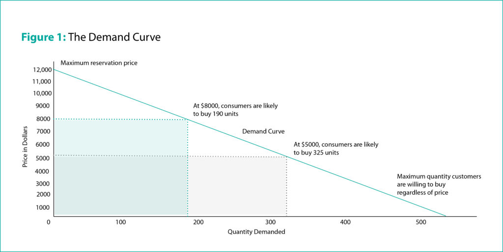
In the linear representation of the demand curve given above, price is plotted on the vertical axis (Y-axis) and quantity on the horizontal axis (X-axis). The downward curve (from left to right) shows the negative relationship between price and quantity purchased by the consumer.
The point of intersection where the Y-axis and the demand curve meet denotes the point at which customers refuse to purchase the product or service because of its high price. This point represents the upper limit of a customer’s capacity to spend.
Similarly, the point where the demand curve intersects with the X-axis indicates the price point at which the customer will purchase a maximum quantity of the product. This marks the upper limit of the quantity demanded by the customer.
In most cases, the demand curve is linear and the slope represents the measures of quantities purchased at various prices. The slope can be calculated using the formula given below.

But, what does this mean?
Let’s take a deep dive into the implications of this formula.
What is Price Elasticity of Demand?
A common sense approach to pricing indicates that more people will buy a product or service when it is priced cheaper than if it is expensive. However, pricing of a product is not as straightforward and simple as it is expected to be. It is affected by the numerous factors that influence a customer’s decision to purchase.
Before fixing a product’s price, we need to understand how elastic or inelastic the product is, how sensitive or insensitive it is to price fluctuations, whether it is a necessity or a luxury, and more. This is where the concept of Price Elasticity of Demand comes into play.
Price elasticity refers to how much of a change in quantity customers will purchase with respect to every change in price. It is the measure of the reaction of a customer to a change in product or service price and can be calculated using the following formula:
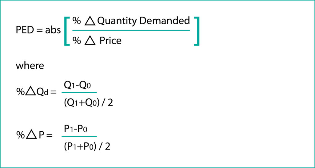
Where:
Qd is the percentage of change in quantity demanded
P is the percentage of change in price
Both Qd and P can be calculated using the formula given below
Qd = (New Quantity – Old Quantity)/Average Quantity
P = (New Price – Old Price)/Average Price
The price elasticity of demand (PED) is also called the elasticity coefficient. It is always negative in value due to the inverse relationship between change in quantity for a given change in price. However, it is represented as an absolute positive value as economists and business people are more concerned about the magnitude of the value calculated than whether it has a positive or negative value. Just because a decrease in quantity occurs, it doesn’t mean that a corresponding decrease in revenue has occurred. Since revenue is the product of price times quantity, an increase in price and profit margin can sufficiently offset the decline caused in purchase volume.
Computing Price Elasticity of Demand
Let’s consider the example of a clothing company. Imagine that the company raised the price of one of its coats from $120 to $140. The percentage change in price can be calculated as follows:
Final price – earlier price/ average price
= $140-$120/($140+$120)/2
= 20/ 130
= 15%
Imagine that the increase in price caused the sale of coats to drop from 1200 to 800 coats.
The percentage change in quantity can be calculated as follows:
Final quantity – earlier quantity/ average quantity
= 800-1200/ (800+1200)/2
= 400/1000
=40%
Plugging these numbers into the PED formula, we get
Price elasticity of demand = Percentage change in quantity demanded/ percentage change in price
= -40/15
= 2.66
But what does that number mean? Let’s find out.
Types of Elasticity
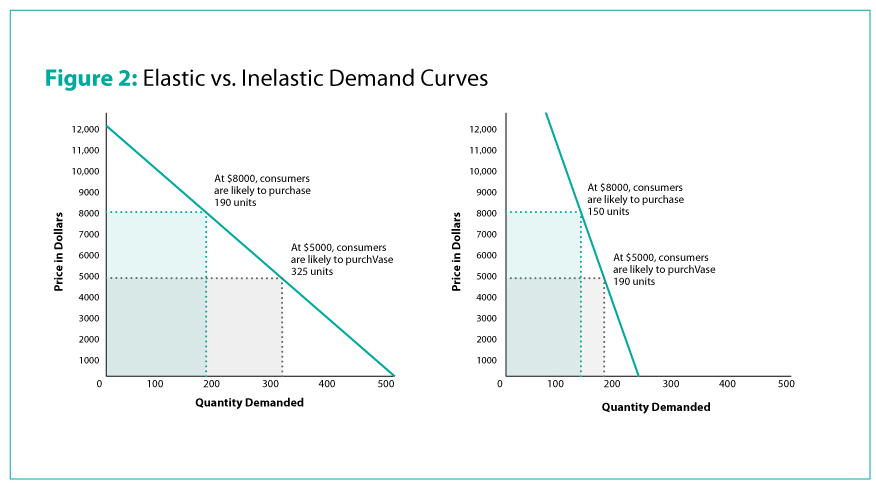
Demand is elastic when a slight change in price results in a disproportionately large variation in the quantity demanded. Similarly, demand is inelastic when the change in price results in a disproportionately smaller variation in quantity demanded. Between elasticity and inelasticity lies the point of unit elasticity where a change in price is reciprocated with a proportionate change in quantity demanded.
So what does the calculated PED value mean?
A PED value of less than 1 shows that the demand for a product is inelastic (not much variation in quantity purchased with an increase or decrease in price). On the other hand, a PED value of more than 1 shows that the demand for a product is elastic (there is significant variation in the quantity of product purchased with changes in price). Thus, a PED value of less than 1 shows a demand for a product that is not price sensitive while a PED value of more than 1 represents demand for a product that is price sensitive.
When the demand for a product (PED) is 1, it means that the product is unit elastic. Theoretically, revenue is maximized when PED is unit elastic.
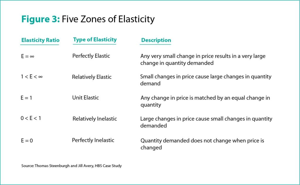
Thomas Steenburgh, a senior lecturer at Darden School of Business, and Jill Avery, a senior lecturer at Harvard Business School, have outlined primarily five zones of elasticity which are given below.
Let’s study these zones of elasticity in detail.
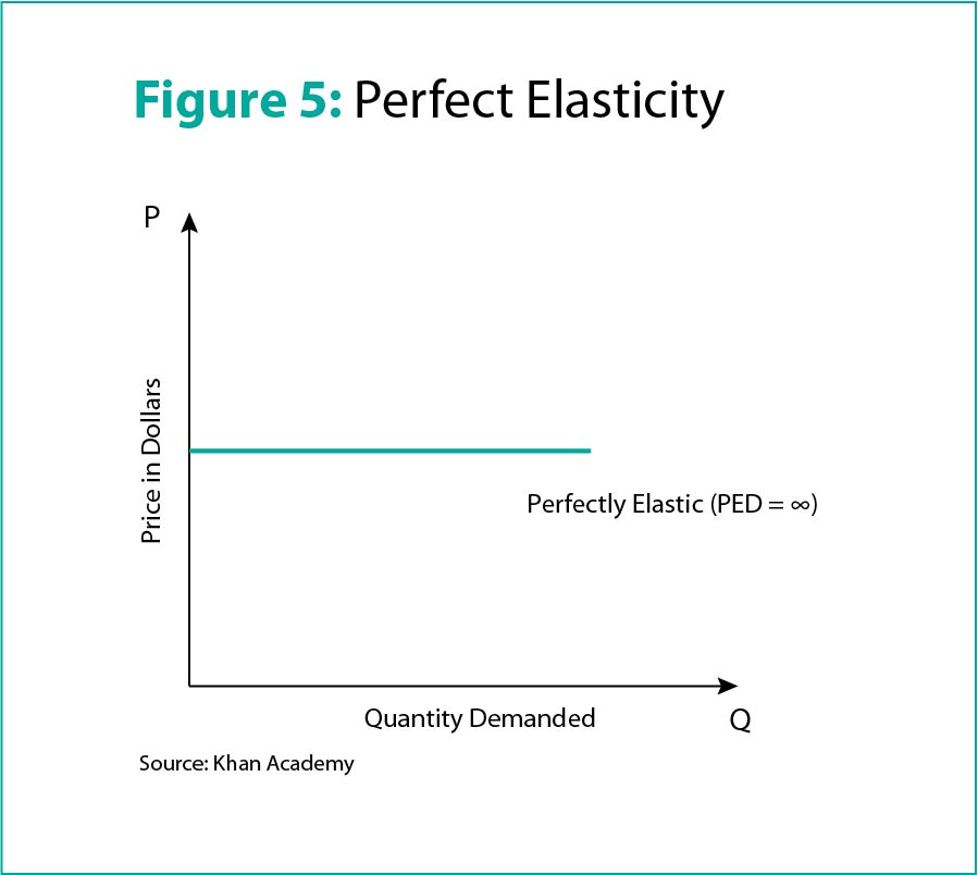
Perfectly Elastic:
When a tiny change in price results in a infinitesimally large change in the quantity demanded, demand is said to be perfectly elastic. Perfect elasticity occurs in situations where the product does not have memorable branding, has several similarly-priced substitutes in the market, and its customers have no particular preference for it.
Let us consider two vending machines (Machine A and Machine B) in a hospital, both containing coke and located adjacent to each other. In a perfect world, the coke in both vending machines will be priced the same (at $1 per bottle). Let’s assume that the daily sales of coke in both machines is 100 bottles each giving us a total of 200 bottles per day.
Now consider a new scenario where the price of coke in Machine A changes to $0.99 while the coke in Machine B remains $1. Assuming that all other factors remain the same (i.e. there is no overcrowding at Machine A or presence of other machines in the vicinity), all the customers intending to purchase coke will opt to buy from Machine A. Thus the daily sales at Machine A will double (go from 100 to 200) while the daily sales at Machine B will fall to zero for a mere change in price by 1 cent.
Now imagine another scenario where the price of coke in Machine A is increased by 1 cent bringing it to $1.01 while the price of coke in Machine B remains $1. Assuming that all other factors remain the same, all the customers will purchase from Machine B making the quantity purchased from Machine A zero for a mere price increase of 1 cent.
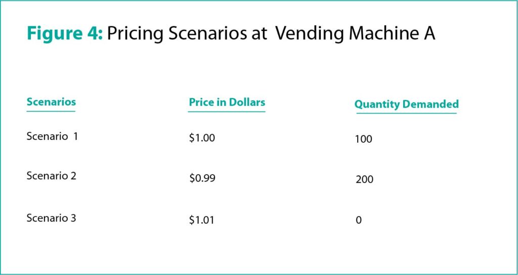
It is evident from the above scenarios that a small price variation of 1 cent brought about a disproportionate change in the quantity of coke demanded at Machine A. If the data obtained from these scenarios is plotted on a graph, the demand demand curve generated will look almost like a straight line.
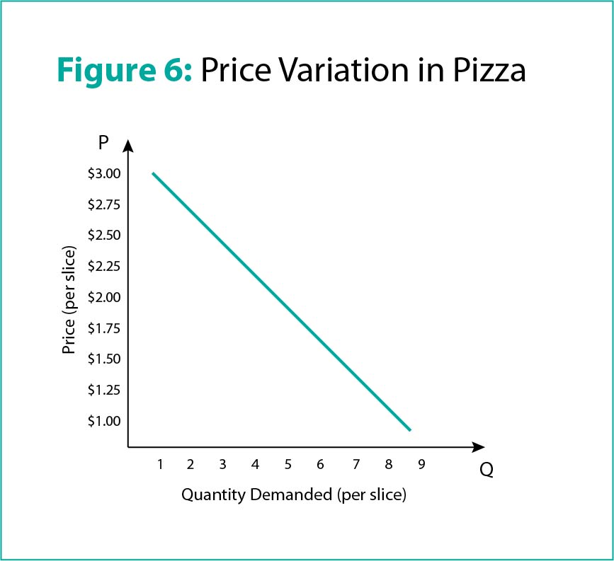
Relatively Elastic
When minor changes in price result in large and disproportionate changes in the quantity of a product purchased, demand is said to be relatively elastic. Consider the example of beef. When the price of beef goes up, consumers generally turn to other meat alternatives like chicken or pork, causing a steep decline in demand for beef. A similar decline in demand is seen when the price of fashion items and restaurant meals are increased (provided that cheaper alternatives are available to consumers). These kinds of products are said to be price-sensitive in nature.
The graph given below shows the decline in demand for pizza with every $0.25 increase in price per slice. It shows that even a minor change in price causes the demand for pizza to decline.
Unit Elastic
Demand for a product is unit elastic when the calculated Price Elasticity of Demand is one. This means that the percentage of change in price and the corresponding percentage change in quantity are the same. Though this concept exists theoretically, it is much harder to find examples of it in the market.
Consider the example of an umbrella manufacturer. If the price of an umbrella was increased from $90 to $100 resulting in a decrease in quantity demand from 1000 umbrellas to 900 umbrellas, then the percentage increase in price will be 10% and the percentage decrease in umbrellas will also be 10%. Thus, the price elasticity of demand for umbrellas will be 1, that is, unit elastic.
Relatively Inelastic
When the calculated value of PED is less than one, it signifies that a change in price of a commodity doesn’t bring about a significant change in quantity demanded.
Consider the example of gasoline. Since most people are dependent on it for commuting from home to work and for transporting goods, a hike in price won’t affect demand much. Only when the rates become exorbitant will there be a considerable lowering in demand.
The graph given below has been created from the data obtained from Boston’s MBTA (Massachusetts Bay Transportation Authority). It shows that the hike in price of gasoline did not significantly change the quantity purchased by any of the organizations.

Relative inelasticity occurs when the product is either an essential commodity or is the product of a premium brand. According to Avery, building brand equity is a good investment as it makes demand for the brands products stronger and more inelastic.
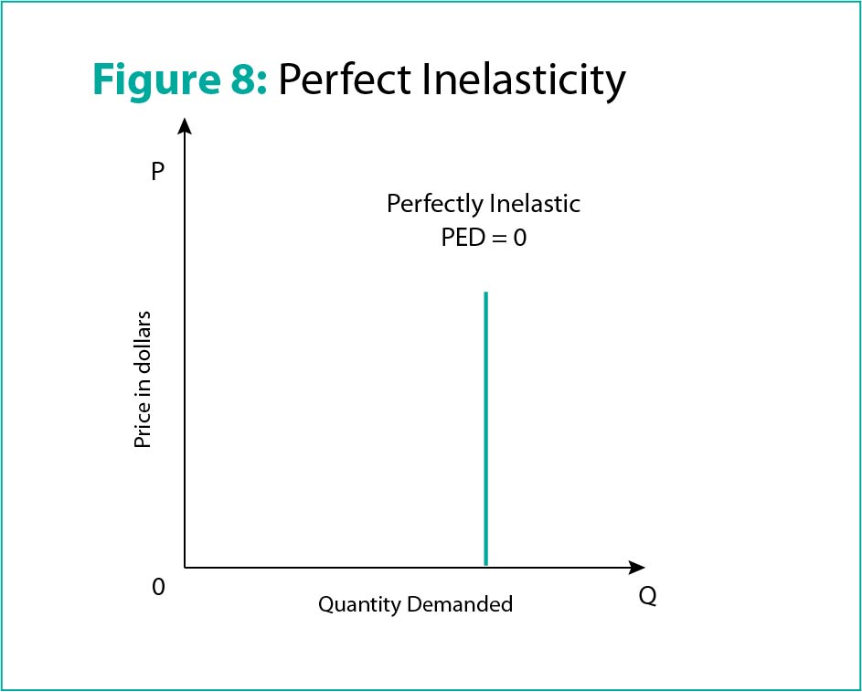
Perfectly Inelastic
In situations where a change in price does not affect the quantity in demand, PED is perfectly inelastic. This means that the commodity is not price-sensitive. This usually happens when a company has a monopoly on the product in demand. Therefore, no matter how much they increase their price, customers will be forced to purchase from them. This is usually seen when the commodity is an essential like water or medication.
Consider the example of a pharmaceutical company that is the only source of a life-saving medication. No matter how much they increase the price of the product, consumers will purchase from them making the product perfectly inelastic. That is, zero fluctuation in quantity purchased with increase in price.
Price Elasticity Along a Linear Demand Curve
How is price elasticity of demand affected towards the end of the demand curve?
The value of PED greatly depends on the nature of the curve being studied. When demand curves are linear in nature, the absolute value of PED falls from the left of the graph to the right. The midpoint of the linear curve is where unit elasticity or PED=1 occurs.
With reference to the graph given below, you can see that, the lower the price of a product, the higher its demand and the lower its PED value will be.
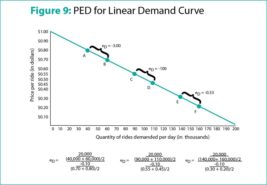
In the above linear demand curve, the absolute price elasticity of demand between the two points A and B is calculated to be 3.00. At this point, a small change in price ($0.10) results in a large change in the quantity purchased (20,000). Thus, when the price is high in the upper left portion of the linear curve, for every minimal percentage change in price, a relatively large change occurs in the quantity purchased. Therefore the absolute value of price elasticity of demand will also be high.
Unit elasticity resides at the midpoint of the linear curve. This is theoretically the optimal point where quantity demanded and price are balanced to obtain maximum profit.
As we move further down the curve and more to the right, we notice that equal changes along the graph represent smaller changes in quantity demanded and larger changes in price. This causes the absolute value of price elasticity of demand to fall.
Let’s consider the price elasticity of demand between points E and F. Here, the price is nearing its lowest point, and demand is nearing its highest point causing price elasticity of demand to fall to 0.33.
When measuring price elasticity of demand along a linear graph, the values vary depending on the interval from which measurements are taken. For every linear demand curve, the value of price elasticity of demand falls as we move down along the curve.
Demand Curves with Constant Price Elasticity
The graphs below show four demand curves that have constant values of price elasticity of demand along all points.
Vertical
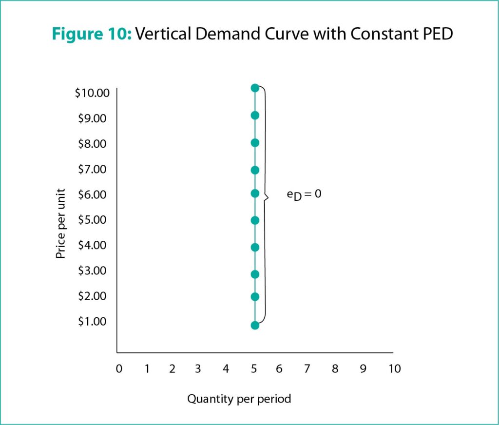
In the first graph, the demand curve is vertical signifying that there is no change to the quantity demanded. Since the percentage of change in quantity is zero for every change in price, the numerator of price elasticity of demand becomes zero. Thus, the value of price elasticity of demand is zero, that is, it is perfectly inelastic. Though it exists theoretically, no natural instance with matching empirical evidence has been found. The only example that has come close is the demand for insulin. Though demand doesn’t increase with decrease in price of insulin, patients consistently consume the quantity needed to keep the disease under control.
Horizontal
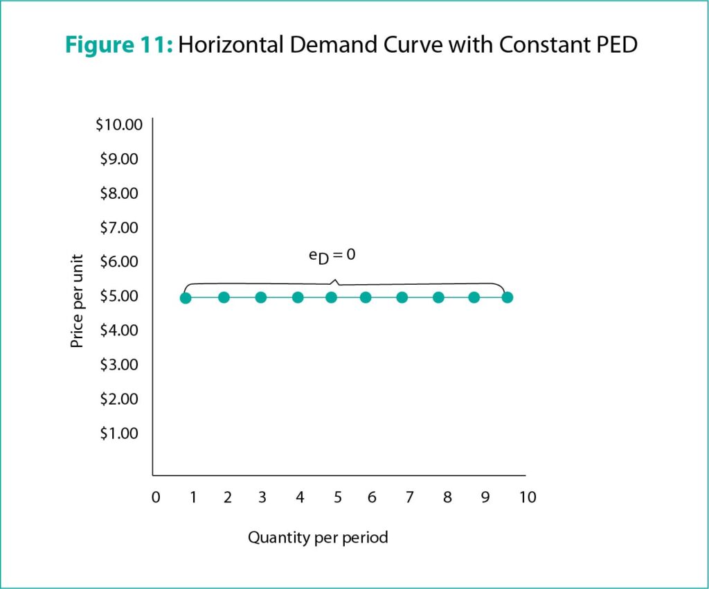
In this demand curve, even the slightest change in price causes an enormous change in the quantity demanded. Thus the change in price in such graphs is negligible causing the denominator of the price elasticity of demand to be zero. In such cases, the value of price elasticity of demand is infinite and the curve is perfectly elastic. This is commonly found in the sales of standardized products such as wheat. If all the other wheat farms are selling a bushel at $4, then a farm can sell as much as they want at $4. However, if the farm increases their price to even $4.01, demand will go down to zero. Also, when the standard price is $4, the farm has no reason to offer pricing below that benchmark.
Non-linear Demand Curves
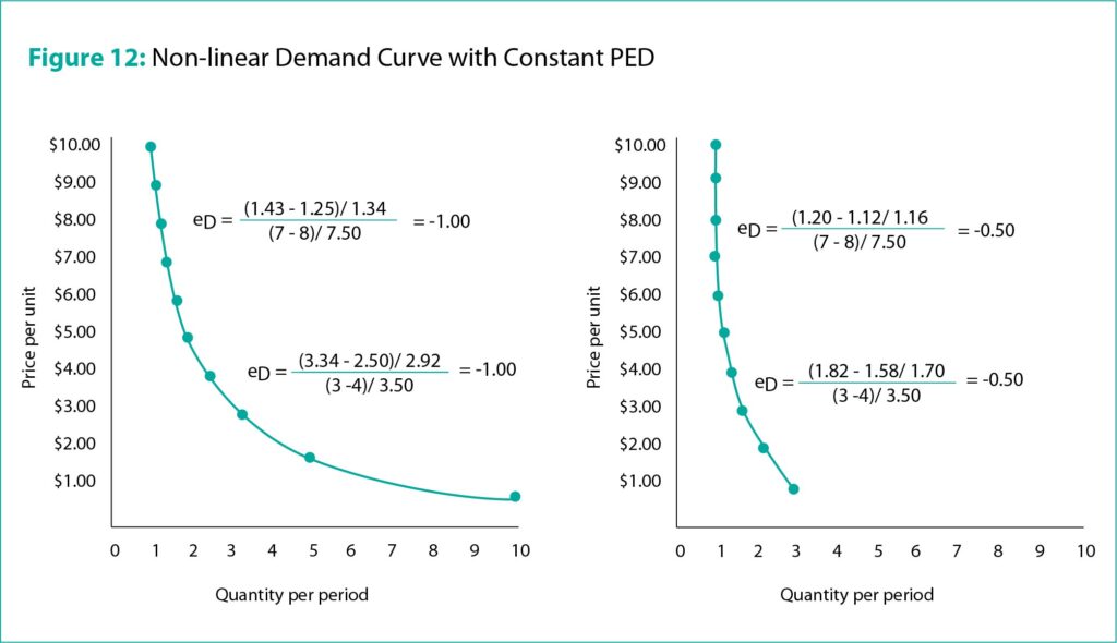
In the nonlinear curves represented above, the price elasticity values are negative, however, the values are also constant throughout the demand curve. In the case of graph A, price elasticity is always constant at -1.00 while in B, price elasticity is constant at -0.5.
Price Elasticity of Demand and Change in Total Revenue
What kind of relationship exists between PED and total revenue? Can the relationship be used to predict the total revenue generated? Let’s explore.
Imagine that a public transit authority is planning to raise its fares. They would first need to find out if the intended hike in price would cause revenue to rise or fall. To determine this, they would first need to calculate the Total Revenue. This is done by multiplying its fare with the total number of passengers commuting.
To enunciate the concept, let’s consider Figure 9 once again.

When the price is $0.80 (point A), the transit authority sells a maximum of 40,000 rides in a day. Total revenue for that instance will be $32,000, that is, 40,000 times $0.80. If the price was lowered to $0.70 (point B) by a reduction of $0.10, then the quantity demand would increase to 60,000 rides with a total revenue of $42,000 ($0.70 multiplied by 60,000). In this scenario, a reduction in fare resulted in an increase in revenue.
However, if the initial price of a ride had been $0.30 (point E) and the transit authority had reduced it to $0.20 (point F) with a price reduction of $0.10 per ride, then the total revenue would fall from $42,000 ($0.30 times 140,000) to $32,000 ($0.20 times 160,000).
Thus, it is evident that the change in revenue depends on the initial price and the original elasticity.
A fact to take note of is that price and quantity carry an inverse relationship. For every increase in price, the quantity demanded goes down and vice versa. Since the total revenue generated is calculated by multiplying price and quantity, it becomes difficult to predict if an increase in price will cause a subsequent increase in revenue or the opposite.
Let us consider the following three examples of price increases to illustrate the case—gasoline, pizza, and diet cola.
Scenario 1: Gasoline
If the daily demand for gasoline at a price of $4.00 per gallon is 1000 gallons, then the total revenue for the day is $4000 ($0.40 times 1000). Imagine that the price of gasoline was increased the next day to $4.25 reducing the demand for gasoline to 950 gallons. The total revenue in the second scenario would be $4037.50, that is, higher than in the first scenario. Thus, though the price of gasoline was increased by 0.25 and resulted in a decline in demand, the higher price compensated for the dip in demand giving an overall increase in revenue.
Scenario 2: Pizza
Let’s consider the pizza sales at an Italian restaurant next. Imagine that the weekly demand is 1000 pizza’s at a price of $9 per pizza. The total revenue generated for the week will be $9000 ($9 times 1000). If the restaurant decides to increase the price of pizza to $10 resulting in a decline in demand to 900 pizzas per week, the total revenue would still be $9000 ($10 times 900). Here the decline in demand is offset by the increase in price such that no change occurs in the total revenue generated.
Scenario 3: Diet Cola
Let’s consider the final example of diet cola. If at the price of $0.50 per can, a total of 1000 cans are purchased daily, then the total revenue for the day is $500 ($0.50 times 1000). Suppose the price of a can of diet cola is increased to $0.55 resulting in a lowered demand of 880 cans per day, the daily total revenue becomes $484 ($0.55 times 880). In this scenario, the reduction in price causes a drop in total revenue.
To summarize, in all three scenarios, the price was increased resulting in a decrease in demand. However, in the first scenario (gasoline), the price rise resulted in an increase in revenue. In the second (pizza) the price rise brought about no change in total revenue and in the third scenario (diet cola), the price increase caused total revenue to decline. What could be the reason? These cases illustrate that the total revenue generated is dependent on the price elasticity of demand.
How can the rise or fall in total revenue be predicted using the price elasticity of demand? The principle is that total revenue will tend toward the same direction of the variable (price or quantity) that has the highest percentage change. If the variables (price and quantity) have the same percentage of change, then total revenue remains constant.
Let us use the three scenarios given above to illustrate this.
Scenario 1: Gasoline
In the earlier scenario, initially, 1000 gallons of gasoline were purchased daily at $4.00 per gallon. This was then increased to $4.25 bringing demand down to 950 gallons per day.
The percentage of change in quantity demanded = difference in quantity/ average quantity
= 950-1000/ (950+1000)/2
= -5.1%
Similarly the percentage of change in price = difference in price/ average price
= 4.25-4/ (4.25+4)/2
= 6.06%
Since the change in percentage of price is greater than the change in percentage of quantity, the total revenue will follow the same trend as the price in this instance. That is, the total revenue will increase just like the price increased.
In this scenario, the price elasticity of demand is calculated as follows
PED = percentage change of quantity/ percentage change in price
= -5.1%/6.06%
= -.084
Thus, we can infer that when the price elasticity of demand tends toward inelasticity, the total revenue either increases with an increase in price or decreases with a decrease in price.
Scenario 2: Pizza
Let’s consider the pizza scenario once again. Initially, 1000 pizzas were sold per week at a price of $9 per pizza. The price was later increased to $10 causing quantity to fall to 900 per week.
Let us calculate the percentage change in quantity demanded.
= 900-1000/(900+1000)/2
= -100/950
= 10.5%
The percentage change of price can be calculated as:
= 10-9/(10+9)/2
= 1/9.5
= 10.5%
Since both percentage change in quantity and price are the same, demand is unit price elastic. Therefore, total revenue remains unchanged.
Scenario 3: Diet Cola
Let’s consider the last scenario where initially, 1000 cans of cola were sold daily at $0.50 per can. An increase in price to $0.55 caused the demand to drop to 880 cans per day.
The percentage change in quantity demanded is
= 880-1000/(880+1000)/2
= 12.8%
The percentage change of price can be calculated as:
= 0.55-0.50/(0.55+0.50)/2
= 9.5%
Since here, the percentage change in quantity is higher than the percentage change in price, the total revenue will follow the same trend as the quantity demanded. That is, when quantity purchased reduces, the total revenue also reduces.
The price elasticity of this particular scenario can be calculated as follows:
= 12.8/9.5
= 1.3
Thus, we can conclude that when demand for a product is elastic, the total revenue follows the same trend as the change in quantity observed.
The relationship between PED and total revenue has been concisely illustrated in the table below.
Factors that Affect Price Elasticity of Demand
Substitutes
A product or service will show great elasticity of demand if there are many substitutes available in the market. When a manufacturer increases the price of their product, customers will switch to other providers that offer the same product at a lower price. For example, if the price of Ford automobiles goes up, customers will choose from other alternatives such as Chevrolets, Toyotas, and more. Thus the price of these segments of automobiles are price elastic.
Goods can also be considered in the form of complements. Goods that are usually consumed together (example, car and petrol) show positive cross-elasticity of demand, that is, their price increases nearly simultaneously causing demand to fall together. On the other hand, substitutes of a product (example, bottled water vs tap water) show negative cross-elasticity of demand, that is, the rise of price in one causes the demand for the other to rise.
Necessity
When a commodity is a necessity, consumers tend to buy it even if the price goes up. Examples of necessities are gasoline and medication. In both cases, even if the price is hiked, consumers will purchase it signifying inelastic demand. On the other hand, products such as chocolate or a cruise to the Bahamas are optional and can be done without. Due to this, a slight increase in price can cause the demand to drop, sending people searching for alternatives or leading them to the decision to do without the product.
Habit-forming
Demand for a product changes according to the taste and preference of the consumer. This is why every year billions of dollars are spent on advertising and marketing to shift customer perception toward a brand. Consumers develop an affinity towards products for several reasons: quality, ideology, reputation, features, and more. When a customer develops the habit of using a certain product, they generally do not mind an increase in price nor do they go searching for substitutes.
Product Price
This doesn’t refer to the price of a product in comparison with competitor pricing. Rather, it refers to the pricing that is generally used for a particular type of good or service. For example, consider two products—a car and a pack of pens. No matter how cheaply a car is priced, it will still cost several thousand dollars. A pack of pens on the other hand costs around 10 dollars. If the pen manufacturer offers a discount of 10% on a pack of pens, you would hardly notice the difference. On the other hand, if the car manufacturer offers a reduction by 10%, that will certainly catch your attention.
Playing on this perception of pricing, Zipcar offers car rentals at daily and hourly rates. When compared with the price of the car, the rental rates appear very attractive.
Purchasing Power
One of the reasons why price hikes should be carefully thought through before implementation is because it can alter the purchasing capacity of a customer. If the price of the good or service goes above the household budget allocated for that particular product, plans to purchase it may end up on the back burner. So, it is crucial to understand the purchasing capacity of your target consumer market before enforcing a price hike.
For example, if you were planning to purchase four pairs of jeans and 4 packs of pens in September, only to find out that the price of both products had doubled, you are more likely to continue buying 4 packs of pens because it doesn’t significantly impact your household budget. However, you might consider purchasing only two pairs of jeans that year as your household budget isn’t flexible enough to accommodate it.
Scarcity
The demand for a product is strongly linked to the length of time for which it is available. Products that are available for only a limited time generally experience demand inelasticity. This means that even if the product price is on the higher side, customers will still buy it. An example to consider is the time-restricted online sales of popular mobile phones. The perceived scarcity of the product drives up demand.
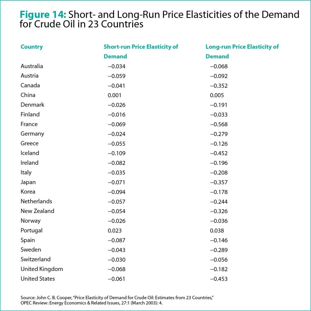
The extent to which scarcity of a product affects demand depends on how long consumers get to prepare for the change. For example, if there is an electricity shortage and prices are raised, most consumers will continue with the higher tariff. However, if the price hike is announced one year in advance, some of the consumers will seek energy alternatives such as installing solar panels on their rooftop. Thus price is generally inelastic over a short period of time, but tends towards elasticity as time passes.
During the period of 171-2000, economist John C. B. Cooper conducted a study on the short and long run price elasticities of demand of crude oil across 23 industrialized countries. He observed that in almost every nation, the values of price elasticity were negative. However, he observed that the absolute values of long-run price elasticities were greater than short-run elasticities. This study was later showcased in an OPEC (Organization of Petroleum Exporting Countries) published journal showing that OPEC not only produced around 45% of the world’s crude oil, but also manipulated price hikes by restricting supply. This not only increased OPECs revenue, it also increased the revenue of other oil producers.
Future Value
Customers are generally more willing to pay for a commodity if they believe that its value will significantly increase in the future. This perception of future value drives up demand for the product. An example of this are investments on vintage cars or in real estate. People often purchase investment properties with the intention of making a profit out of its sale in the future.
Thus, consumer psychology and trends can make consumers perceive even basic consumer goods as an investment.
How Companies Use Price Elasticity of Demand
Now that we have reviewed what price elasticity of demand means, how it can be calculated, and what factors influence it, let’s explore how companies make use of PED.
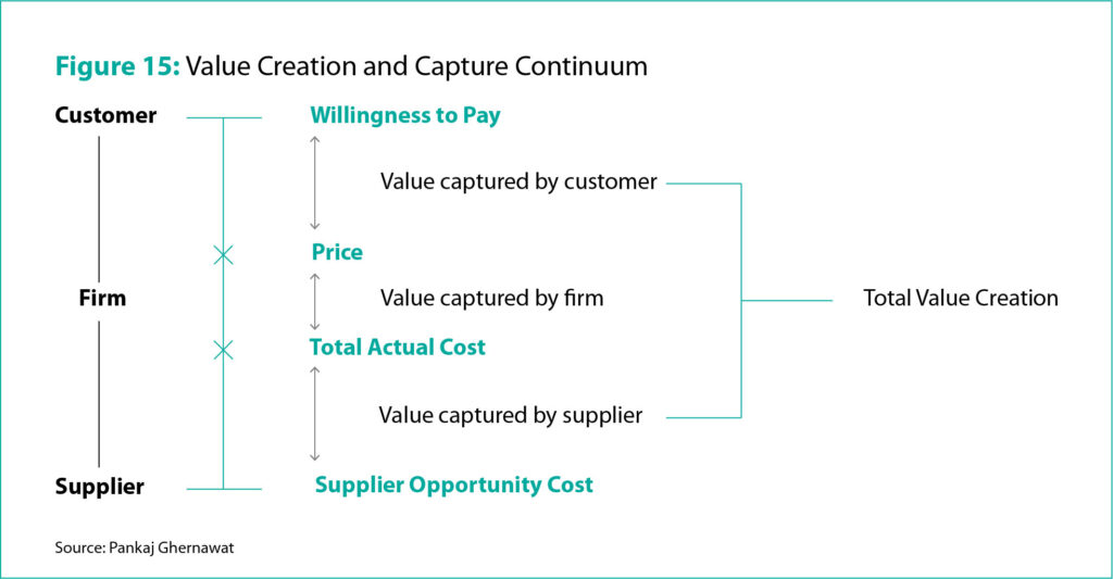
The function of a company is twofold. The first is to create value for its customers and the second is to capture value for its stakeholders. The former is done by producing a good/ service that provides value to customers and the latter is done through profits generated by employing various pricing strategies. In simple terms, the core function of a company is to maximize profit.
So, what is the role of a marketer within an organization? They are also concerned with the maximization of profit for the organization. Since they are not directly involved in manipulating costs, they accomplish their objective by maximizing revenue. For this, they make use of the 4 P’s of marketing: Product, Price, Place, and Promotion. Here, product refers to the nature and differentiating features of a good/service. Price refers to the amount for which the product is sold. Place talks about how easily the good/ service can be accessed. Finally, promotion refers to the various methods employed to inform customers about the benefits of the good or service.
In order to do this, the marketer estimates demand, studies the price elasticities of different price combinations, and uses data to advise management on optimal pricing and promotion strategies. Since price elasticity in the real world is dynamic and complex with various tangible and intangible factors influencing demand, predicting optimal pricing often becomes a challenging task.
According to Avery, when demand for a product is highly elastic, it indirectly means that the product has been accepted as a commodity by consumers. Though beginning with elasticity is fine, a marketers ultimate goal is to shift demand toward inelasticity. This can be done by creating products that are meaningful and differentiated enough to increase a consumer’s desire to purchase the product regardless of price.
Price elasticity of demand should constantly be monitored as increased elasticity means that either a competitor that offers a comparable substitute has entered the market or that a consumer’s purchasing capacity has gone down. In both cases, suitable adjustments have to be made to maintain a company’s market share.
PED can be calculated only after the price of a commodity has been increased or decreased in the market and the resultant shift in sales has been quantified. Since it is not advisable for companies to proceed with price changes without first studying the market, they often gather data from smaller focus groups through detailed questionnaires that capture the customers’ general sentiment toward the price change.
Common Mistakes when using PED
According to Jill Avery, many managers are misguided by their assumption that their experience in pricing is enough to determine a price change to which customers will respond. However, rarely do they test extreme price changes on consumers. In most cases, they collect responses from a small sample of consumers to price changes that range between 5-20% of an increase or decrease. Since price elasticity of demand is a dynamic concept, it’s impact on a multivariate market is not easy to predict. What if we leave the price of a commodity the same year on year? There too, the myriad factors influencing price elasticity play a role. Just because customers have been willing to pay a certain price over the years doesn’t mean that they will continue to be willing tomorrow.
Therefore, market price elasticity extrapolated from surveys need not be accurate as consumers may say that they are willing to pay, but may not when the price hike rolls up. According to Jill Avery, it is far more accurate to run an in-market A/B test where the product is introduced at the new price point and the difference in demand between the new and old price points can be compared. Now that the world is digital, this is relatively easier as you can increase the price of a product online to $15 for about 10 minutes, quickly return it to the old $7, and assess the consumer response to both.
Pricing strategy requires a keen understanding of consumer behavior. Price elasticity of demand calculations and market tests can only quantify variations, they cannot provide explanations why consumers are acting a certain way. Therefore, quantification should be supplemented with additional qualitative research that can shed light on consumer behavior.
Knowing the price elasticity of demand of a product alone doesn’t show you how to manage the price points. Instead a deeper understanding of the current demand elasticity and the factors influencing them toward elastic or inelastic scenarios should be cultivated. Since the market is ever-changing and complex, this study will have to be constantly updated so that you can adjust pricing and introduce differentiations to make your product accessible, affordable, and valuable to consumers.
Applications of Price Elasticity of Demand
While price elasticity of demand is used primarily as a predictive tool, it also has other applications. It is widely used as a lag indicator that provides information on how companies are performing across various parameters. These could be product performance, competitor and complement performance, branding or marketing performance, or even macroeconomic health.
Product Performance
The goal of every company is to produce products or services that have a unique differentiating factor and offer sustainable value to their customers. The greater the product differentiation, the higher the consumer’s willingness to purchase it and the larger the value of its demand inelasticity.
Price elasticity of demand is thus both an effective indicator as well as measure of the real or perceived uniqueness of a product in the marketplace.
Competitor and Complement Performance
Price elasticity of demand is also a good indicator of competitive intensity of substitutes and complements in the market. When PED is elastic, it means that either competition within the product genre is very high at that price point or that the cost of complements is rising.
Branding/ Marketing Performance
Even if there is no true differentiating factor between a product and its substitutes, creating the perception of a uniqueness through effective branding strategies in itself plays an important role in consumer adoption. Thus, price elasticity can be used as a scale to measure the comparative brand equity of a company with its competitors. Products with high elasticity scores indicate weak branding or poor differentiation, leaving room for alternative products to gain market share.
Product/ Business Lifecycle
According to Joel Deal’s HBR article on new product pricing policies, price elasticity can be used to accurately gauge a company’s level of maturity. This depends on three clear-cut elements:
a. Technical Maturity
A product reaches technical maturity when product development declines, standardization of features and performance occurs among other brands, and customer expectations out of the product stabilizes. The longer a product spends time on the market, the more it grows toward technical maturity.
b. Market Maturity
A product reaches market maturity when consumers accept the product, the service it provides, its value proposition, and have trust that the stabilized product will perform satisfactorily.
c. Competitive Maturity
Competitive maturity occurs when the market share, pricing, and positioning of competitor brands stabilize.
Macroeconomic Health
Finally, price elasticity of demand is also an indicator of the overall health of the economy where the product is sold. This relates to both demographics and the income levels of target consumers. When high-cost products are introduced into low income markets, demand will naturally follow an elastic curve. Similarly, when low cost products are introduced into high income markets, they will yield demand curves that tend toward inelasticity.
Conclusion
Identifying the right price for a product is far from an exact science. Even with tools like price elasticity of demand at disposal for more than a century, marketers have only been able to make rudimentary predictions about future consumer behavior.
In today’s digital age, PED needs to be supplemented with big data analytics and rapid A/B testing. From Uber who uses dynamic price surge features to maintain demand-supply equilibrium real-time to startups like 100% Pure who have successfully increased operating profits by 13.5% over merely three months, companies are not only capable of predicting demand change with every unit change in price with staggering accuracy, they are also able to identify the underlying reasons why.

